
PROJECT 03-02 [Multiple Uses] Histogram Equalization
- Write a computer program for computing the histogram of an image.
- Implement the histogram equalization technique discussed in Section 3.3.1.
- Download Fig. 3.8(a) and perform histogram equalization on it.
As a minimum, your report should include the original image, a plot of its histogram, a plot of the histogram-equalization transformation function, the enhanced image, and a plot of its histogram. Use this information to explain why the resulting image was enhanced as it was.
变换函数是:$s_k=T(r_k)=(L-1)\sum_{j=0}^kp_r(r_j)=(L-1)\sum_{j=0}^k\frac{n_j}{n}$,其中$k=0,1,\ldots,L-1$
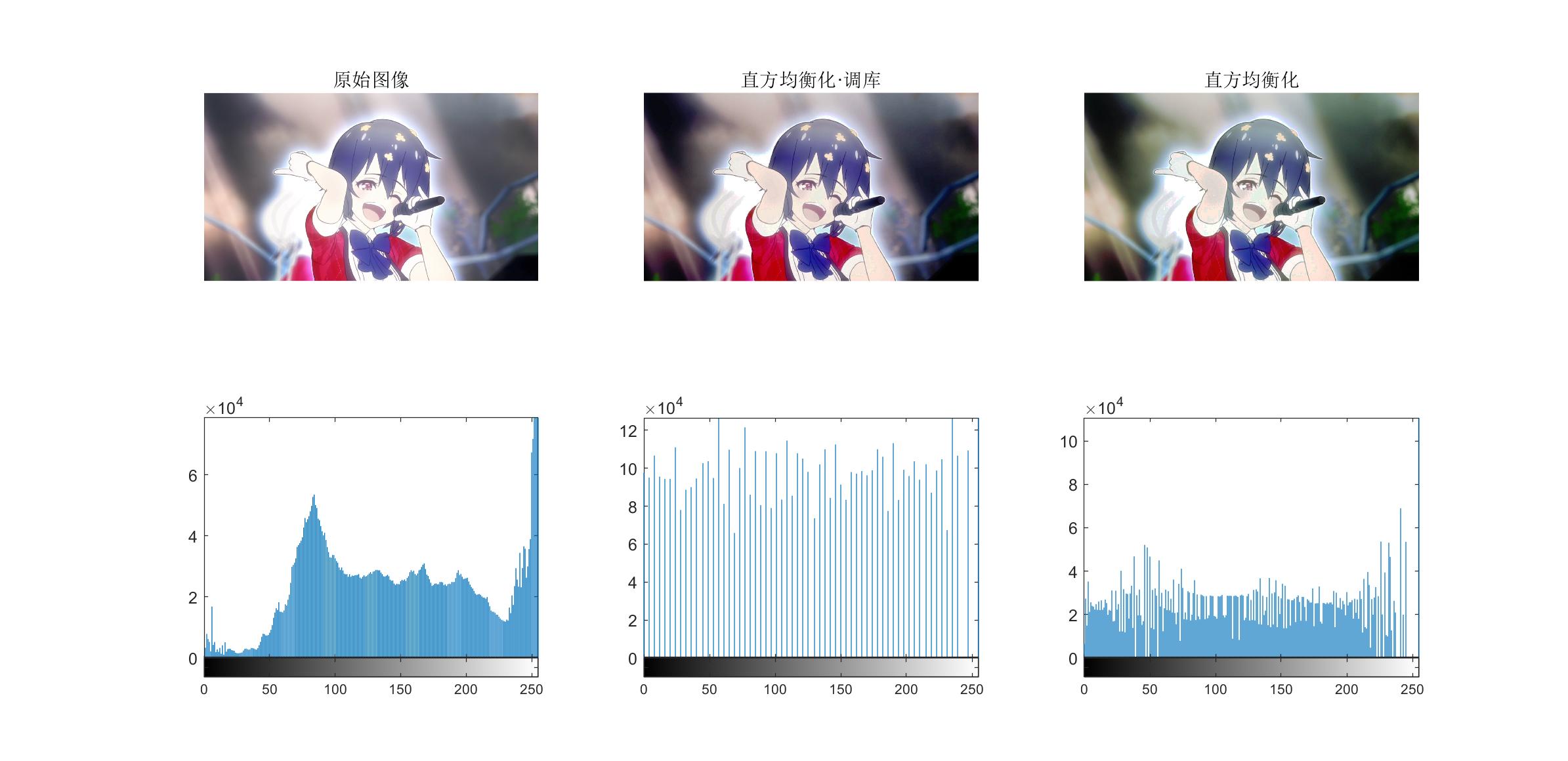
我想做一些加强,针对彩色图片做直方图均衡化。查了一些网上资料,就是对三维RGB图像的三种颜色分别做一次灰度均衡。
    I=imread('MizunoAi.jpg');
    subplot(2,3,1);imshow(I);title('原始图像');subplot(2,3,4);imhist(I);
    c=histeq(I);
    subplot(2,3,2);imshow(c);title('直方均衡化·调库');subplot(2,3,5);imhist(c);
    c=cat(3,histogram(I(:,:,1)),histogram(I(:,:,2)),histogram(I(:,:,3)));
    subplot(2,3,3);imshow(c);title('直方均衡化');subplot(2,3,6);imhist(c);
function J=histogram(I)
    J=I;
    [n,m]=size(I);
    a=zeros(1,256);
    b=zeros(1,256);
    for i=1:n
        for j=1:m
            a(1,I(i,j)+1)=a(1,I(i,j)+1)+1;
        end
    end
    sum=0;
    for i=1:256
        sum=sum+a(1,i);
        b(1,i)=255*sum/(m*n);
    end
    for i=1:n
        for j=1:m
            d=J(i,j)+1;
            J(i,j)=b(1,d);
        end
    end
end
运行结果如下,同时输出调用matlab自己的直方图均衡函数的结果作为对比,发现自己写的图像均衡偏绿…不过右侧阴影处的细节变得清晰了。
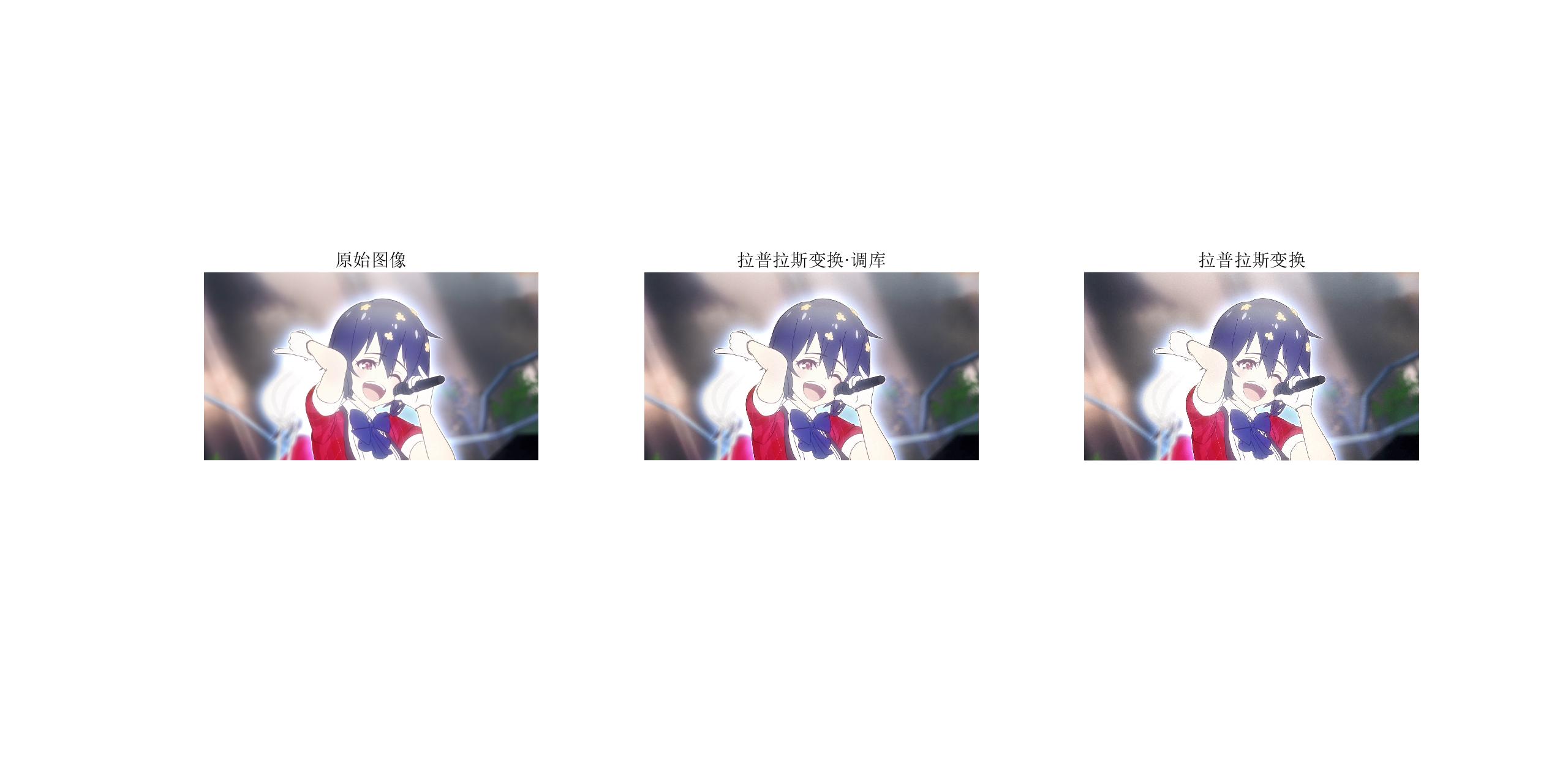
PROJECT 03-05 Enhancement Using the Laplacian
- Use the programs developed in Projects 03-03 and 03-04 to implement the Laplacian enhancement technique described in connection with Eq. (3.7-5). Use the mask shown in Fig. 3.39(d).
- Duplicate the results in Fig. 3.40. You will need to download Fig. 3.40(a).
    clear;clc;
    I=imread('MizunoAi.jpg');
    subplot(1,3,1);imshow(I);title('原始图像');
    c=I-imfilter(I,fspecial('laplacian',0),'replicate');
    subplot(1,3,2);imshow(c);title('拉普拉斯变换·调库');
    c=cat(3,laplacian(I(:,:,1)),laplacian(I(:,:,2)),laplacian(I(:,:,3)));
    subplot(1,3,3);imshow(c);title('拉普拉斯变换');
function J=laplacian(I1)
    I=im2double(I1);
    [m,n]=size(I);
    A=zeros(m,n);
    for i=2:m-1
        for j=2:n-1
            A(i,j)=I(i+1,j)+I(i-1,j)+I(i,j+1)+I(i,j-1)-4*I(i,j);
        end
    end
    J=I-A;
end
运行结果如下,同时输出调用matlab自己的拉普拉斯方法的结果作为对比。
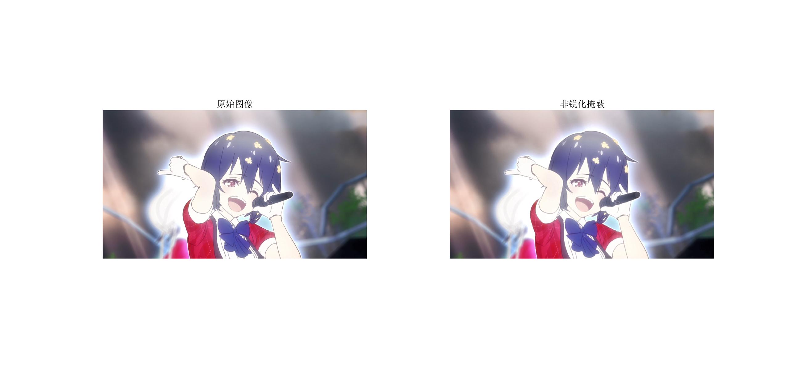
PROJECT 03-06 Unsharp Masking
- Use the programs developed in Projects 03-03 and 03-04 to implement highboost filtering, as given in Eq. (3.7-8). The averaging part of the process should be done using the mask in Fig. 3.34(a).
- Download Fig. 3.43(a) and enhance it using the program you developed in (a). Your objective is to choose constant A so that your result visually approximates Fig. 3.43(d).
这里使用拉普拉斯变换得到模糊图像。
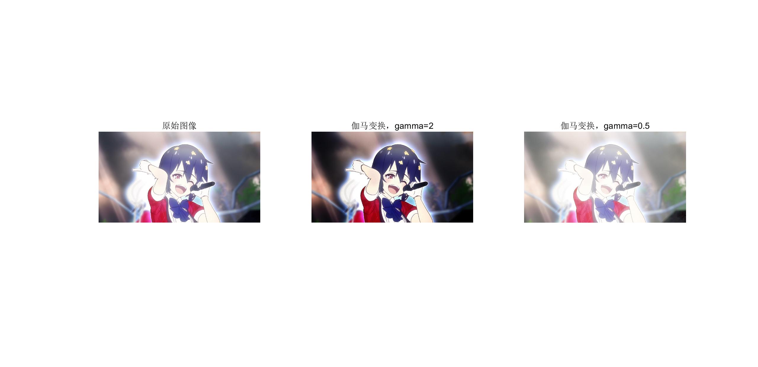
伽马变换
    close all;clc;clear all;
    I=imread('MizunoAi.jpg');
    subplot(1,2,1);imshow(I);title('原始图像');
    c=cat(3,unsharpMasking(I(:,:,1)),unsharpMasking(I(:,:,2)),unsharpMasking(I(:,:,3)));
    subplot(1,2,2);imshow(c);title('非锐化掩蔽');
function J=unsharpMasking(I)
    J = I + imfilter(I, fspecial('laplacian',0));
end
    close all;clc;clear all;
    I=imread('MizunoAi.jpg');
    subplot(1,3,1);imshow(I);title('原始图像');
    c=cat(3,gamma(I(:,:,1),2),gamma(I(:,:,2),2),gamma(I(:,:,3),2));
    subplot(1,3,2);imshow(c);title('伽马变换,gamma=2');
    c=cat(3,gamma(I(:,:,1),0.5),gamma(I(:,:,2),0.5),gamma(I(:,:,3),0.5));
    subplot(1,3,3);imshow(c);title('伽马变换,gamma=0.5');
function J=gamma(I1,g)
    I = double(I1);
    [row,col] = size(I);
    J = zeros(row,col);
    for i = 1:row
        for j = 1:col
            J(i,j) = I(i,j).^g;
        end
    end
    J = mat2gray(J);
end

|

|